Category: DRC+

TL;DR It massively cheats and it’s bad, just ignore it.

First, OAA finally lets us compare all outfielders to each other regardless of position and without need for a positional adjustment.  Range Defense Added unsolves that problem and goes back to comparing position-by-position.  It also produces some absolutely batshit numbers.

From 2022:

Stanton was -2 OAA on the year in ~300 innings (like 1/4th of a season).  An ROS of -21.5 over a full season is equivalent to pushing -50 OAA.  The worst qualified season in the Statcast era is 2016 Matt Kemp (-26 OAA in 240 opportunities), and that isn’t even -*10*% success probability added (analogous to ROS), much less -21.5%.  The worst seasons at 50+ attempts (~300 innings) are 2017 Trumbo and 2019 Jackson Frazier at -12%.  Maybe 2022 Yadier Molina converted to a full-time CF could have pulled off -21.5%, but nobody who’s actually put in the outfield voluntarily for 300 innings in the Statcast era is anywhere near that terrible.  That’s just not a number a sane model can put out without a hell of a reason, and 2022 Stanton was just bad in the field, not “craploads worse than end-stage Kemp and Trumbo” material.

I thought CF was supposed to be the harder position.  No idea where that number comes from.  Barrera has played OF quite well in his limited time, but not +6.1% over the average CF well.

As I did with the infield edition, I’ll be using rate stats (Range Out Score and OAA/inning) for correlations, each player-position-year combo is treated separately, and it’s important to repeat the reminder that BP will blatantly cheat to improve correlations without mentioning anything about what they’re doing in the announcements, and they’re almost certainly doing that again here.

Here’s a chart with year-to-year correlations broken down by inning tranches (weighted by the minimum of the two paired years)

Focus on the left side of the chart first.  OAA/inning behaves reasonably, being completely useless for very small numbers of innings and then doing fine for players who actually play a lot.  ROS is simply insane.  Outfielders in aggregate get an opportunity to make a catch every ~4 innings (where opportunity is a play that the best fielders would have a nonzero chance at, not something completely uncatchable that they happen to pick up after it’s hit the ground).

ROS is claiming meaningful correlations on 1-2 opportunities and after ~10 opportunities, it’s posting year to year correlations on par with OAA’s after a full season.  That’s simply impossible (or beyond astronomically unlikely) to do with ~10 yes/no outcome data points with average talent variation well under +/-10%.  The only way to do it is by using some kind of outside information to cheat (time spent at DH/1B?, who knows, who cares).

I don’t know why the 0-10 inning correlations are so low- those players played a fair bit at other positions (see the right side of the table), so any proxy cheat measures should have reasonably stabilized- but maybe the model is just generically batshit nonsense at extremely low opportunities at a position for some unknown reason as happened with the DRC+ rollout (look at the gigantic DRC+ spread on 1 PA 1 uBB pitchers in the cheating link above).

Also, once ROS crosses the 200-inning threshold, it starts getting actively worse at correlating to itself.  Across all three positions, it correlates much better at lower innings totals and then shits the bed once it starts trying to correlate full-time seasons to full-time seasons.  This is obviously completely backwards of how a metric should behave and more evidence that the basic model behavior here is “good correlation based on cheating (outside information) that’s diluted by mediocre correlation on actual play-outcome data.”

They actually do “improve” on team switchers here relative to nonswitchers- instead of being the worst as they were in the infield, again likely due to overfitting to a fairly small number of players- but it’s still nothing of note given how bad they are relative to OAA’s year-to year for regular players even with the cheating.

Since there’s nothing of any interest going on in the country or the world today, I decided the time was right to defend the honour of a Toronto pitcher from the 80s.  Looking deeper into this article, https://www.baseballprospectus.com/news/article/57310/rubbing-mud-dra-and-dave-stieb/ which concluded that Stieb was actually average or worse rate-wise, many of the assertions are… strange.

First, there’s the repeated assertion that Stieb’s K and BB rates are bad.  They’re not.  He pitched to basically dead average defensive catchers, and weighted by the years Stieb pitched, he’s actually marginally above the AL average.  The one place where he’s subpar, hitting too many batters, isn’t even mentioned.  This adds up to a profile of

Accounting for the extra HBPs, these components account for about 0.05 additional ERA over league average, or ~1%.  Without looking at batted balls at all, Stieb would only be 1% worse than average (AL and NL are pretty close pitcher-quality wise over this timeframe, with the AL having a tiny lead if anything).  BP’s version of FIP- (cFIP) has Stieb at 104.  That doesn’t really make any sense before looking at batted balls, and Stieb only allowed a HR/9 of 0.70 vs. a league average of 0.88.  He suppressed home runs by 20%- in a slight HR-friendly park- over 2900 innings, combined with an almost dead average K/BB profile, and BP rates his FIP as below average.  That is completely insane.

The second assertion is that Stieb relied too much on his defense.  We can see from above that an almost exactly average percentage of his PAs ended with balls in play, so that part falls flat, and while Toronto did have a slightly above-average defense, it was only SLIGHTLY above average.  Using BP’s own FRAA numbers, Jays fielders were only 236 runs above average from 79-92, and prorating for Stieb’s share of IP, they saved him 24 runs, or a 0.08 lower ERA (sure, it’s likely that they played a bit better behind him and a bit worse behind everybody else).  Stieb’s actual ERA was 3.44 and his DRA is 4.43- almost one full run worse- and the defense was only a small part of that difference.  Even starting from Stieb’s FIP of 3.82, there’s a hell of a long way to go to get up to 4.43, and a slightly good defense isn’t anywhere near enough to do it.

Stieb had a career BABIP against of .260 vs. AL average of .282, and the other pitchers on his teams had an aggregate BABIP of .278.  That’s more evidence of a slightly above-average defense, suppressing BABIP a little in a slight hitter’s home park, but Stieb’s BABIP suppression goes far beyond what the defense did for everybody else.  It’s thousands-to-1 against a league-average pitcher suppressing HR as much as Stieb did.  It’s also thousands-to-1 against a league-average pitcher in front of Toronto’s defense suppressing BABIP as much as Stieb did.  It’s exceptionally likely that Stieb actually was a true-talent soft contact machine.  Maybe not literally to his careen numbers, but the best estimate is a hell of a lot closer to career numbers than to average after 12,000 batters faced.

This is kind of DRA and DRC in a microcosm.  It can spit out values that make absolutely no sense at a quick glance, like a league-average K/BB guy with great HR suppression numbers grading out with a below-average cFIP, and it struggles to accept outlier performance on balls in play, even over gigantic samples, because the season-by-season construction is completely unfit for purpose when used to describe a career.  That’s literally the first thing I wrote when DRC+ was rolled out, and it’s still true here.

What does it mean to talk about the uncertainty in, say, a pitcher’s ERA or a hitter’s OBP?  You know exactly how many ER were allowed, exactly how many innings were pitched, exactly how many times the batter reached base, and exactly how many PAs he had.  Outside of MLB deciding to retroactively flip a hit/error decision, there is no uncertainty in the value of the stat.  It’s an exact measurement.  Likewise, there’s no uncertainty in Trout’s 2013 wOBA or wRC+.  They reflect things that happened, calculated in deterministic fashion from exact inputs.  Reporting a measurement uncertainty for any of these wouldn’t make any sense.

The Statcast metrics are a little different- EV, LA, sprint speed, hit distance, etc. all have a small amount of random error in each measurement, but since those errors are small and opportunities are numerous, the impact of random error is small to start with and totally meaningless quickly when aggregating measurements.  There’s no point in reporting random measurement uncertainty in a public-facing way because it may as well be 0 (checking for systematic bias is another story, but that’s done with the intent of being fixed/corrected for, not of being reported as metric uncertainty).

Point 1:

So we can’t be talking about the uncertainties in measuring/calculating these kinds of metrics- they’re irrelevant-to-nonexistent.  When we’re talking about the uncertainty in somebody’s ERA or OBP or wRC+, we’re talking about the uncertainty of the player’s skill at the metric in question, not the uncertainty of the player’s observed value.  That alone makes it silly to report such metrics as “observed value +/- something”, like ERA 0.37 +/- 3.95, because it’s implicitly treating the observed value as some kind of meaningful central-ish point in the player’s talent distribution.  There’s no reason for that to be true *because these aren’t talent metrics*.  They’re simply a measure of something over a sample, and many such metrics frequently give values where a better true talent is astronomically unlikely to be correct (a wRC+ over 300) or even impossible (an ERA below 0) and many less extreme but equally silly examples as well.

Point 2:

Expressing something non-stupidly in the A +/- B format (or listing percentiles if it’s significantly non-normal, whatever) requires a knowledge of the player’s talent distribution after the observed performance, and that can’t be derived solely from the player’s data.  If something happens 25% of the time, talent could cluster near 15% and the player is doing it more often, talent could cluster near 35% and the player is doing it less often, or talent could cluster near 25% and the player is average.  There’s no way to tell the difference from just the player’s stat line and therefore no way to know what number to report as the mean, much less the uncertainty.  Reporting a 25% mean might be correct (the latter case) or as dumb as reporting a mean wRC+ of 300 (if talent clusters quite tightly around 15%).

Once you build a prior talent distribution (based on what other players have done and any other material information), then it’s straightforward to use the observed performance at the metric in question and create a posterior distribution for the talent, and from that extract the mean and SD.  When only the mean is of interest, it’s common to regress by adding some number of average observations, more for a tighter talent distribution and fewer for a looser talent distribution, and this approximates the full Bayesian treatment.  If the quantity in the previous paragraph were HR/FB% (league average a little under 15%), then 25% for a pitcher would be regressed down a lot more than for a batter over the same number of PAs because pitcher HR/FB% allowed talent is much more tightly distributed than hitter HR/FB% talent, and the uncertainty reported would be a lot lower for the pitcher because of that tighter talent distribution.  None of that is accessible by just looking at a 25% stat line.

Actual talent metrics/projections, like Steamer and ZiPS, do exactly this (well, more complicated versions of this) using talent distributions and continually updating with new information, so when they spit out mean and SD, or mean and percentiles, they’re using a process where those numbers are meaningful, getting them as the result of using a reasonable prior for talent and therefore a reasonable posterior after observing some games.  Their means are always going to be “in the middle” of a reasonable talent posterior, not nonsense like wRC+ 300.

Which brings us to DRC+.. I’ve noted previously that the DRC+ SDs don’t make any sense, but I didn’t really have any idea how they were coming up with those numbers until  this recent article, and a reference to this old article on bagging.  My last two posts pointed out that DRC+ weights way too aggressively in small samples to be a talent metric and that DRC+ has to be heavily regressed to make projections, so when we see things in that article like Yelich getting assigned a DRC+ over 300 for a 4PA 1HR 2BB game, that just confirms what we already knew- DRC+ is happy to assign means far, far outside any reasonable distribution of talent and therefore can’t be based on a Bayesian framework using reasonable talent priors.

So DRC+ is already violating point 1 above, using the A +/- B format when A takes ridiculous values because DRC+ isn’t a talent metric.  Given that it’s not even using reasonable priors to get *means*, it’s certainly not shocking that it’s not using them to get SDs either, but what it’s actually doing is bonkers in a way that turns out kind of interesting.  The bagging method they use to get SDs is (roughly) treating the seasonal PA results as the exact true talent distribution of events, drawing  from them over and over (with replacement) to get a fake seasonal line, doing that a bunch of times and taking the SD of the fake seasonal lines as the SD of the metric.

That’s obviously just a category error.  As I explained in point 2, the posterior talent uncertainty depends on the talent distribution and can’t be calculated solely from the stat line, but such obstacles don’t seem to worry Jonathan Judge.  When talking about Yelich’s 353 +/- 6  DRC+, he said “The early-season uncertainties for DRC+ are high. At first there aren’t enough events to be uncertain about, but once we get above 10 plate appearances or so the system starts to work as expected, shooting up to over 70 points of probable error. Within a week, though, the SD around the DRC+ estimate has worked its way down to the high 30s for a full-time player.”  That’s just backwards about everything.  I don’t know (or care) why their algorithm fails under 10 PAs, but writing “not having enough events to be uncertain about” shows an amazing misunderstanding of everything.

The accurate statement- assuming you’re going in DRC+ style using only YTD knowledge of a player- is “there aren’t enough events to be CERTAIN about of much of anything”, and an accurate DRC+ value for Yelich- if DRC+ functioned properly as a talent metric- would be around 104 +/- 13 after that nice first game.  104 because a 4PA 1HR 2BB game preferentially selects- but not absurdly so- for above average hitters, and a SD of 13 because that’s about the SD of position player projections this year.  SDs of 70 don’t make any sense at all and are the artifact of an extremely high SD in observed wOBA (or wRC+) over 10-ish PAs, and remember that their bagging algorithm is using such small samples to create the values.  It’s clear WHY they’re getting values that high, but they just don’t make any sense because they’re approaching the SD from the stat line only and ignoring the talent distribution that should keep them tight.  When you’re reporting a SD 5 times higher than what you’d get just picking a player talent at random, you might have problems.

The Bayesian Central Limit Theorem

I promised there was something kind of interesting, and I didn’t mean bagging on DRC+ for the umpteenth time, although catching an outright category error is kind of cool.  For full-time players after a full season, the DRC+ SDs are actually in the ballpark of correct, even though the process they use to create them obviously has no logical justification (and fails beyond miserably for partial seasons, as shown above).  What’s going on is an example of the Bayesian Central Limit Theorem, which states that for any priors that aren’t intentionally super-obnoxious, repeatedly observing i.i.d variables will cause the posterior to converge to a normal distribution.  At the same time, the regular Central Limit Theorem means that the distribution of outcomes that their bagging algorithm generates should also approach a normal distribution.

Without the DRC+ processing baggage, these would be converging to the same normal distribution, as I’ll show with binomials in a minute, but of course DRC+ gonna DRC+ and turn virtually identical stat lines into significantly different numbers

Ellsbury is a little more TTO-based and gets an 11 SD to Sandoval’s 7.  Seems legit.  Regardless of these blips, high single digits is about right for a DRC+ (wRC+) SD after observing a full season.

Getting rid of the DRC+ layer to show what’s going on, assume talent is uniform on [.250-.400] (SD of 0.043) and we’re dealing with 1000 Bernoulli observations.  Let’s say we observe 325 successes (.325), then when we plot the Bayesian posterior talent distribution and the binomial for 1000 p=.325 events (the distribution that bagging produces)

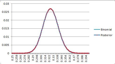
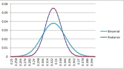
They overlap so closely you can’t even see the other line.  Going closer to the edge, we get, for 275 and 260 observed successes,

At 275, we get a posterior SD of .13 vs the binomial .14, and at 260, we start to break the thing, capping how far to the left the posterior can go, and *still* get a posterior SD of .11 vs .14.  What’s going on here is that the weight for a posterior value is the prior-weighted probability that that value (say, .320) produces an observation of .325 in N attempts, while the binomial bagging weight at that point is the probability that .325 produces an observation of .320 in N attempts.  These aren’t the same, but under a lot of circumstances, they’re pretty damn close, and as N grows, and the numbers that take the place of .320 and .325 in the meat of the distributions get closer and closer together, the posterior converges to the same normal that describes the binomial bagging.  Bayesian CLT meets normal CLT.

When the binomial bagging variance starts dropping well below the prior population variance, this convergence starts to happen enough to where the numbers can loosely be called “close” for most observed success rates, and that transition point happens to come out around a full season of somewhat regressed observation of baseball talent. In the example above, the prior population SD was 0.043 and the binomial variance was 0.014, so it converged excellently until we ran too close to the edge of the prior.  It’s never always going to work, because a low end talent can get unlucky, or a high end talent can get lucky, and observed performance can be more extreme than the talent distribution (super-easy in small samples, still happens in seasonal ones) but for everybody in the middle, it works out great.

Let’s make the priors more obnoxious and see how well this works- this is with a triangle distribution, max weight at .250 straight line down to a 0 weight at .400.

290 successes, .0143 vs .0140

325 successes, .0144 vs .0148

350 successes, .0143 vs .0151

350 successes, .0143 vs .0151

325 successes, .0144 vs .0148

290 successes, .0143 vs .0140

The left-weighted prior shifts the means, but the standard deviations are obviously about the same again here.  Let’s up the difficulty even more, starting with a N(.325,.020) prior (0.020 standard deviation), which is pretty close to the actual mean/SD wOBA talent distribution among position players (that distribution is left-weighted like the triangle too, but we already know that doesn’t matter much for the SD)

360 successes, .012 vs .015

325 successes, .012 vs .015

290 successes, .012 vs .013

Even now that the bagging distributions are *completely* wrong and we’re using observations almost 2 SD out, the standard deviations are still .014-.015 bagging and .012 for the posterior.  Observing 3 SD out isn’t significantly worse.  The prior population SD was 0.020, and the binomial bagging variance was 0.014, so it was low enough that we were close to converging when the observation was in the bulk of the distribution but still nowhere close when we were far outside, although the SDs of the two were still in the ballpark everywhere.

Using only 500 observations on the N(.325,.020) prior isn’t close to enough to pretend there’s convergence even when observing in the bulk.

The posterior has narrowed to a SD of .014 (around 9 points of wRC+ if we assume this is wOBA and treat wOBA like a Bernoulli, which is handwavy close enough here), which is why I said above that high-single-digits was “right”, but the binomial variance is still at .021, 50% too high.  The regression in DRC+ tightens up the tails compared to “binomial wOBA”, and it happens to come out to around a reasonable SD after a full season.

Just to be clear, the bagging numbers are always wrong and logically unjustified here, but they’re a hackjob that happens to be “close” a lot of the time when working with the equivalent of full-season DRC+ numbers (or more).  Before that point, when the binomial bagging variance is higher than the completely naive population variance (the mechanism for DRC+ reporting SDs in the 70s, 30s, or whatever for partial seasons), the bagging procedure isn’t close at all.  This is just another example of DRC+ doing nonsense that looks like baseball analysis to produce a number that looks like a baseball stat, sometimes, if you don’t look too closely.

This is a cut-out from a longer post I was running some numbers for, but it’s straightforward enough and absurd enough that it deserves a standalone post.  I’d previously looked at DRAA linear weights and the relevant chart for that is reproduced here.  This is using seasons with 400+PA.

I reran the same analysis on 2019 YTD stats, with all position players and with a 25 PA minimum, and these are the values I recovered.  Full year is the new DRAA row above, and the percentages are the percent relative to those values.

So.. this is quite something.  First of all, events are “more-than-half-deserved” relative to the full season after only 25-50 PA.  There’s no logical or mathematical reason for that to be true, for any reasonable definition of “deserved”, that quickly.  Second, BIP hits are discounted *LESS* in a small sample than walks are, and BIP outs are discounted *LESS* in a small sample than strikeouts are.  The whole premise of DRC+ is that TTO outcomes belong to the player more than the outcomes of balls in play, and are much more important in small samples, but here we are, with small samples, and according to DRC+, the TTO OUTCOMES ARE RELATIVELY LESS IMPORTANT NOW THAN THEY ARE AFTER A FULL SEASON.  Just to be sure, I reran with wRAA and extracted almost the exact same values as chart 1, so there’s nothing super weird going on here.  This is complete insanity- it’s completely backwards from what’s actually true, and even to what BP has stated is true.  The algorithm has to be complete nonsense to “come to that conclusion”.

Reading the explanation article, I kept thinking the same thing over and over.  There’s no clear logical or mathematical justification for most steps involved, and it’s just a pile of junk thrown together and tinkered with enough to output something resembling a baseball stat most of the time if you don’t look too closely. It’s not the answer to any articulable, well-defined question.  It’s not a credible run-it-back projection (I’ll show that unmistakably in the next post, even though it’s already ruled out by the.. interesting.. weightings above).

Whenever a hodgepodge model is thrown together like DRC+ is, it becomes difficult-to-impossible to constrain it to obey things that you know are true.  At what point in the process did it “decide” that TTO outcomes were relatively less important now?  Probably about 20 different places where it was doing nonsense-that-resembles-baseball-analysis and optimizing functions that have no logical link to reality.  When it’s failing basic quality testing- and even worse, when obvious quality assurance failures are observed and not even commented on (next post)- it’s beyond irresponsible to keep running it out as something useful solely on the basis of a couple of apples-to-oranges comparisons on rigged tests.

BP released an update to DRC+ yesterday purporting to fix/improve several issues that have been raised on this blog.  One thing didn’t change at all though- DRC+ still isn’t a hitting metric.  It still assigns pitchers artificially low values no matter how well they hit, and the areas of superior projection (where actually true) are largely driven by this.  The update claimed two real areas of improvement.

Valuation

The first is in treating outlier players.  As discussed in C’mon Man- Baseball Prospectus DRC+ Edition by treating player seasons individually and regressing them, instead of treating careers, DRC+ will continually fail to realize that outliers are really outliers. Their fix is, roughly, to make a prior distribution based on all player performances in surrounding years, and hopefully not regress the outliers as much because it realizes something like them might actually exist.  That mitigates the problem a little, sometimes, but it’s still an essentially random fix.  Some cases previously mentioned look better, and others, like Don Kessinger vs. Larry Bowa still don’t make any sense at all.  They’re very similar offensive players, in the same league, overlapping in most of their careers, and yet Kessinger gets wRC-DRC bumped from 72 to 80 while Bowa only goes from 70 to 72, even though Kessinger was *more* TTO-based.

To their credit- or at least to credit their self-awareness, they seem to know that their metric is not reliable at its core for valuation.  Jonathan Judge says

“As always, you should remember that, over the course of a career, a player’s raw stats—even for something like batting average—tend to be much more informative than they are for individual seasons. If a hitter consistently seems to exceed what DRC+ expects for them, at some point, you should feel free to prefer, or at least further account for, the different raw results.”

Roughly translated, “Regressed 1-year performance is a better estimation of talent that 1-year raw performance, but ignoring the rest of a player’s career and re-estimating talent 1 year at a time can cause discrepancies, and if it does, trust the career numbers more.” I have no argument with that.  The question remains how BP will actually use the stat- if we get more fluff pieces on DRC+ outliers who are obviously just the kind career discrepancies Judge and I talked about, that’s bad.  If it is mainly used to de-luck balls in play for players who haven’t demonstrated that they deserve much outlier consideration, that’s basically fine and definitely not the dumbest thing I’ve seen lately.

This, on the other hand, well might be.

Not just the blatant cheating (Gathright is the only position player on the list), but the DRC+ SDs make no sense.  Based on one identical PA, DRC+ claims that there’s a 1 in hundreds of thousands chance that Runzler is a better hitter than Melancon and also assigns negative runs to a walk because a pitcher drew it.  The DRC+ SDs were pure nonsense before, but now they’re a new kind of nonsense. These players ranged from 9-31 SD in the previous iteration of DRC+, and while the low end of that was still certainly too low, SDs of 1-2 are beyond absurd, and the fact that they’re that low *only for players with almost no PAs* is a huge red flag that something inside the black box is terribly wrong.  Tango recently explored the SD of wRC+/WAR and found that the SDs should be similar for most players with the same number of PA.  DRC+ SDs done correctly could legitimately show up as slightly lower, because they’re the SD of a regressed stat, but that’s with an emphasis on slightly.  Not SDs of 1 or 2 for anybody, and not lower SDs for pitchers and part-time players who aren’t close to a season full of PAs.

Park Adjustments

I’d observed before that DRC+ still contains a lot of park factor and they’ve taken steps to address this.  They adjusted Colorado hitters more in this iteration while saying there wasn’t anything wrong with their previous park factors.  I’m not sure exactly how that makes sense, unless they just weren’t correcting for park factor before, but they claim to be park-isolated now and show a regression against their park factors to prove it.  Of course the key word in that claim is THEIR park factors.  I reran the numbers from the linked post with the new DRC+s, and while they have made an improvement, they’re still correlated to both Fangraphs park factor and my surrounding-years park factor estimate at the r=0.17-0.18 level, with all that entails (still overrating Rockies hitters, for one, just not by as much).

A reader saw a television piece on DRC+, googled and found this site, and asked me a simple question: how does a DRC+ value correlate to a win? I answered that privately, but it occurred to me that team W-L record was a simple way to test DRC+’s claim of superior descriptiveness without having to rely on its false claim of being park-adjusted.

I used seasons from 2010-2018, with all stats below adjusted for year and league- i.e. the 2018 Braves are compared to the 2018 NL average.  Calculations were done with runs/game and win% since not all seasons were 162 games.

Run differential is cheating of course, since it’s the only one on the list that knows about runs allowed, but it does show that at the seasonal level, scoring runs and not allowing them is the overwhelming driver of W-L record and that properly matching RS to RA- i.e. not losing 5 1-run games and winning a 5-run game to “balance out”- is a distant second.

Good offense is based on three major things- being good, sequencing well, and playing in a friendly park.  Only the first two help you to outscore your opponent who’s playing the game in the same park, and Runs Scored can’t tell the difference between a good offense and a friendly park.  As it turns out, properly removing park factor noise (wRC+) is more important than capturing sequencing (Runs Scored).

Both clearly beat wOBA, as expected, because wRC+ is basically wOBA without park factor noise, and Runs Scored is basically wOBA with sequencing added.  OBP beating wOBA is kind of an accident- wOBA *differential* would beat OBP *differential*- but because park factor is more prevalent in SLG than OBP, offensive wOBA is more polluted by park noise and comes out slightly worse.

And then there’s DRC+.  Not only does it not know sequencing, it doesn’t even know what component events (BB, 1B, HR, etc) actually happened, and the 25% or so of park factor that it does neutralize is not enough to make up for that.  It’s not a good showing for the fancy new most descriptive metric ever when it’s literally more valuable to know a team’s OBP than its DRC+ to predict its W-L record, especially when wRC+ crushes the competition at the same task.